Methodology
Proposed Debiasing Inference Procedure
Consider the observed data \(\{(Y_i,R_i,X_i)\}_{i=1}^n \subset \mathbb{R}\times \{0,1\} \times \mathbb{R}^d\), where \(Y_i\) is the outcome variable that could be missing, \(R_i\) is the binary variable indicating the missingness of \(Y_i\), and \(X_i\) is the fully observed high-dimensional covariate vector for \(i=1,...,n\).
Our proposed debiasing method aims at conducting valid statistical inference on the linear regression function \(m_0(x)=\mathrm{E}(Y|X=x)=x^T\beta_0\) under the “missing at random (MAR)” assumption. Specifically, the method consists of the following procedures.
Step 1: Compute the Lasso pilot estimate \(\widehat{\beta}\) of the regression coefficient using the complete-case data as:
where \(\lambda >0\) is a regularization parameter.
Step 2: Obtain consistent estimates \(\widehat{\pi}_i, i=1,...,n\) of the propensity scores \(\pi_i = \mathrm{P}(R_i=1|X_i)\) by any machine learning method (not necessarily a parametric model) applied on the data \(\{(X_i,R_i)\}_{i=1}^n \subset \mathbb{R}^d \times \{0,1\}\). See the scikit-learn package and the related probability calibration for potential propensity score estimation methods.
Step 3: Solve for the debiasing weight vector \(\widehat{\mathbf{w}}\equiv \widehat{\mathbf{w}}(x) = \left(\widehat{w}_1(x),...,\widehat{w}_n(x)\right)^T \in \mathbb{R}^n\) through a debiasing program defined as:
\[\min_{\mathbf{w}\equiv \mathbf{w}(x) \in \mathbb{R}^n} \left\{\sum_{i=1}^n \widehat{\pi}_iw_i(x)^2: \left\|x- \frac{1}{\sqrt{n}}\sum_{i=1}^n w_i(x)\cdot \widehat{\pi}_i\cdot X_i \right\|_{\infty} \leq \frac{\gamma}{n} \right\},\]
where \(\gamma >0\) is a tuning parameter.
Step 4: Define the debiasing estimator for \(m_0(x)\) as:
Step 5: Construct the asymptotic \((1-\alpha)\)-level confidence interval for \(m_0(x)\) as:
where \(\Phi(\cdot)\) denotes the cumulative distribution function (CDF) of \(\mathcal{N}(0,1)\). If \(\sigma_{\epsilon}^2\) is unknown, then it can be replaced by any consistent estimator \(\widehat{\sigma}_{\epsilon}^2\).
For the implementation of this package Debias-Infer, we fit the Lasso pilot estimate \(\widehat{\beta}\) in Step 1 by the scaled Lasso [2] so as to automatically select the regularization parameter \(\lambda >0\) and simultaneously produce a consistent estimator of the noise level \(\sigma_{\epsilon}^2\).
As for solving the debiasing program in Step 3, we leverage the CVXPY package. To select the tuning parameter \(\gamma >0\), we use the cross-validation on the dual formulation of the debiasing program as:
This dual program is solved via the coordinate descent algorithm [3] in our package.
In the reference paper [1], we prove that the confidence interval in Step 5 is asymptotically valid and our debiased estimator in Step 4 is semi-parametrically efficient among all asymptotically linear estimators with MAR outcomes; see Figure 1 for how our debiased estimator performs (under two different rules for the cross-validation) when compared with the Lasso estimate.
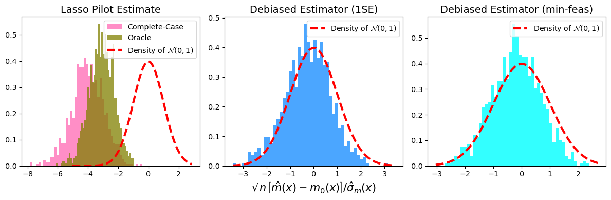
Figure 1: Comparison of our debiased estimators under two different choices of the tuning parameters (“1SE” and “min-feas”) with the conventional Lasso estimates based on complete-case or oracle data.